How does qPCR work: SYBR® Green vs TaqMan®
Written by Éva Mészáros
11. May 2022
qPCR, or real-time PCR, is a widely used method to quantify DNA sequences in samples. This article gives you a comprehensive introduction to the topic, explaining how dye-based and probe-based qPCR assays (like SYBR Green and TaqMan) work, how to validate your amplification experiments, and how to analyze your qPCR data.
Table of contents
qPCR vs PCR vs RT-PCR
Before explaining how qPCR works, we would like to briefly outline its difference from standard PCR and RT-PCR.
Whereas standard PCR monitors DNA amplification upon reaction completion, qPCR uses fluorescent signals to monitor DNA amplification as the reaction progresses. This is why qPCR is also referred to as real-time PCR, quantitative PCR or quantitative real-time PCR.
RT-PCR, not to be confused with real-time PCR, stands for reverse transcription PCR and can be used to amplify RNA target sequences. It involves an initial incubation of the sample RNA with a reverse transcriptase enzyme and a DNA primer before amplification.
For more detailed definitions of the different types of PCR, please refer to our blog post 'The complete guide to PCR'.
How qPCR works
qPCR relies on fluorescence from intercalating dyes or hydrolysis probes to measure DNA amplification after each thermal cycle. The most common dye-based method is SYBR Green, and the most common probe-based method is TaqMan, which is why this article will focus on these two qPCR techniques. If you wish, you can also watch our video explaining how the different methods work, including the advantages and disadvantages of each.
SYBR Green qPCR
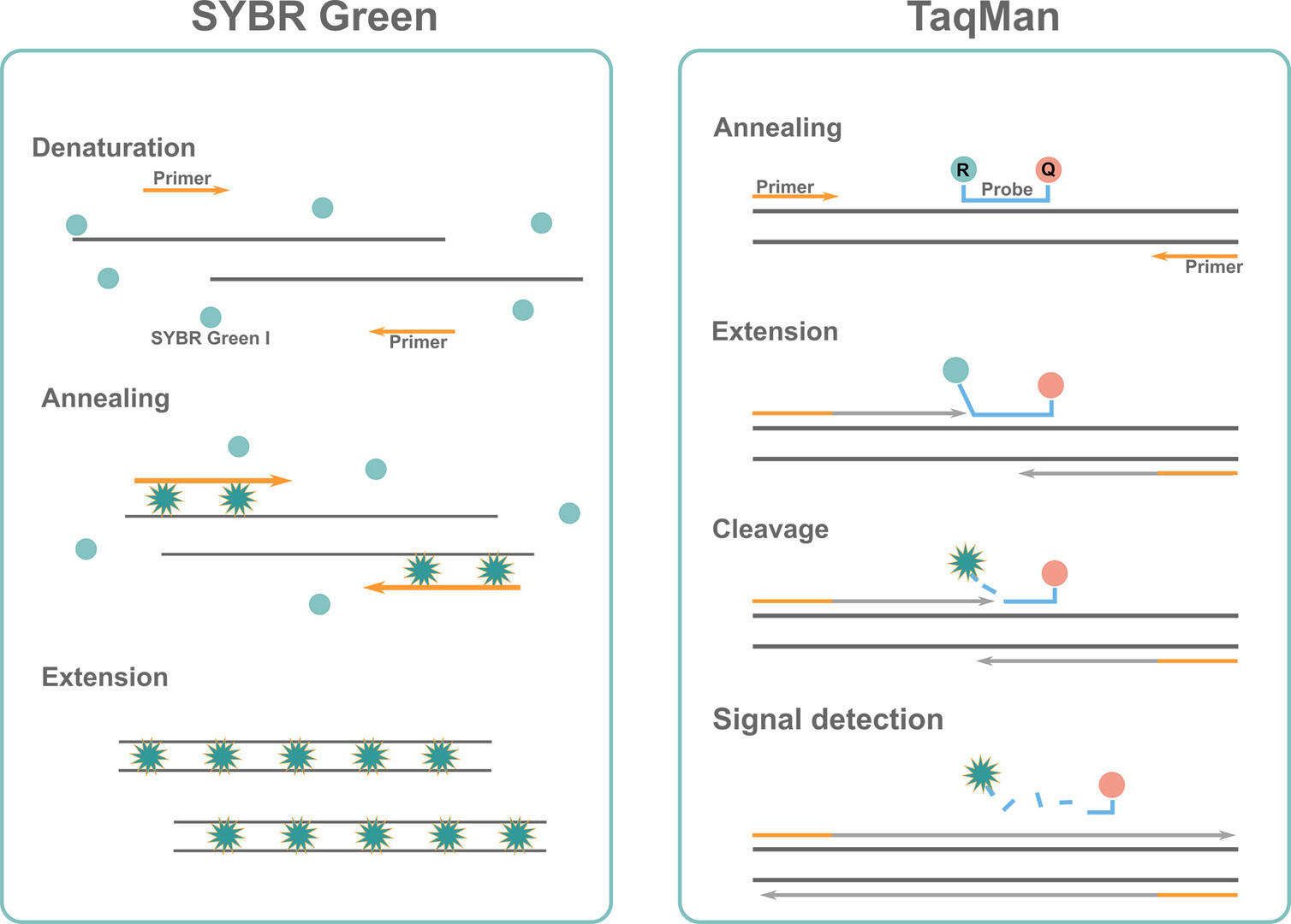
Like standard PCR, the SYBR Green protocol consists of denaturation, annealing and extension phases. The difference being that you add some double-stranded DNA binding dye, SYBR Green I, to your master mix during qPCR setup. This fluorescent dye intercalates into double-stranded DNA sequences during the extension phase, where it shows a strong increase in fluorescent signal. Measuring this signal at the end of every thermal cycle will allow you to determine the quantity of double-stranded DNA present.
The downside of the SYBR Green assay is that the dye binds to any double-stranded DNA sequence. This means that you could also detect fluorescence emitted from non-specific qPCR products, such as primer dimers. To eliminate this risk, check the reaction specificity by performing a melting curve analysis, explained later in the article, or use the TaqMan method.
TaqMan qPCR
Instead of using intercalating dyes, this assay uses TaqMan probes with a 5' fluorescent reporter dye and a 3' quencher dye. These probes are target-specific, and only bind to the DNA sequence of interest downstream of one of the primers during the annealing step. When the enzyme Taq polymerase encounters the TaqMan probe during the extension phase, it displaces and cleaves the 5' reporter dye. Once the reporter dye has been separated from the quencher dye, its measurable fluorescent signal at the end of every qPCR cycle increases significantly. The second DNA strand is synthesized in parallel but, as no probe is attached to it, this process can't be monitored by fluorescence measurements.
Compared to the SYBR Green assay, the use of TaqMan probes is more expensive, but also offers two significant advantages:
- the TaqMan assay only measures amplification progression of the target sequence, as the probes are target specific.
- you can monitor the quantity of various qPCR products in a single reaction by adding different primers and TaqMan probes with different reporter dyes to the master mix. This multiplex approach allows you to detect several fluorescent signals at the end of every thermal cycle.
Amplification plot
For both qPCR methods, data is visualized in an amplification plot, with the number of thermal cycles on the x-axis, and the fluorescent signals detected on the y-axis:
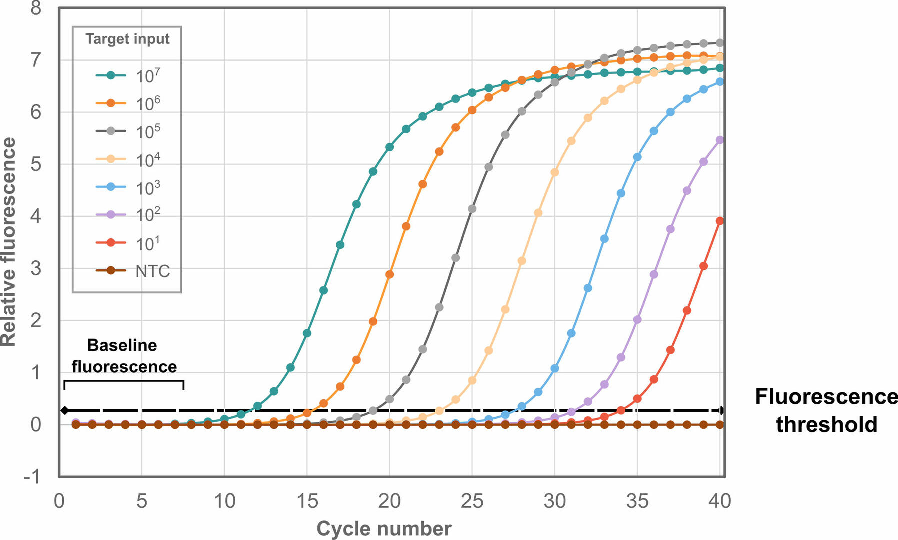
As can be seen, fluorescence remains at background levels during the first thermal cycles. Eventually, the fluorescent signal reaches the fluorescence threshold, where it is detectable over the background fluorescence. The cycle number at which this happens is called the threshold cycle (Ct). If the Ct value for a sample is high, it means that little starting material was present, and vice versa. Please note that you should always analyze at least three replicates of each sample, as tiny pipetting errors during qPCR set-up can result in huge differences in Ct values.
The Ct value is sometimes also referred to as crossing point (Cp), take-off point (TOP) or quantification cycle (Cq) value, with MIQE guidelines suggesting using Cp value to standardize terminology.1 In this article we will continue to call it Ct, as this is the most commonly used term.
MIQE guidelines
The MIQE (Minimum Information for Publication of Quantitative Real-Time PCR Experiments) guidelines describe the minimum information necessary for evaluating qPCR experiments. When publishing a manuscript, the scientist needs to provide all relevant experimental conditions and assay characteristics described by the MIQE guidelines, allowing reviewers to assess the validity of the protocols used, and enabling other scientists to reproduce the experiments.
Validation of qPCR assays
qPCR amplification plots can be analyzed using absolute or relative quantification. However, before explaining qPCR data analysis, we need to quickly discuss how to determine reaction efficiency and specificity. You don't need to perform these steps after every qPCR experiment, but should always validate these two values when setting up a new qPCR protocol or changing your current workflows.
Reaction efficiency
A perfect qPCR assay would have a reaction efficiency of 100 %, which means that the number of template DNA copies would double at every thermal cycle. As this is almost impossible to achieve in practice, reaction efficiencies between 90 and 110 % are considered to be ideal.
To calculate the reaction efficiency of your assay, you need to set up a 10-fold serial dilution of an undiluted sample with a known amount of template DNA. After running a qPCR, create a standard curve with the log of the starting quantity on the x-axis and the Ct values on the y-axis.
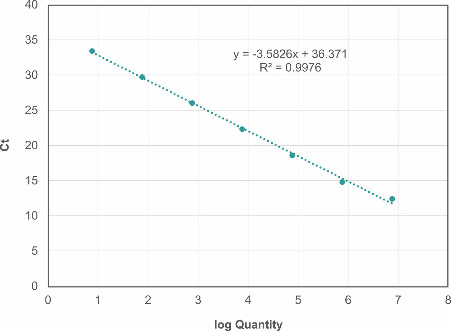
Using the equation for the linear regression line (y = mx + b), you can now determine the reaction efficiency as follows2:
Efficiency = (10(-1/m)-1) x 100
In our example, m would be -3.5826, resulting in a reaction efficiency of 90.1634 %.
Reaction specificity
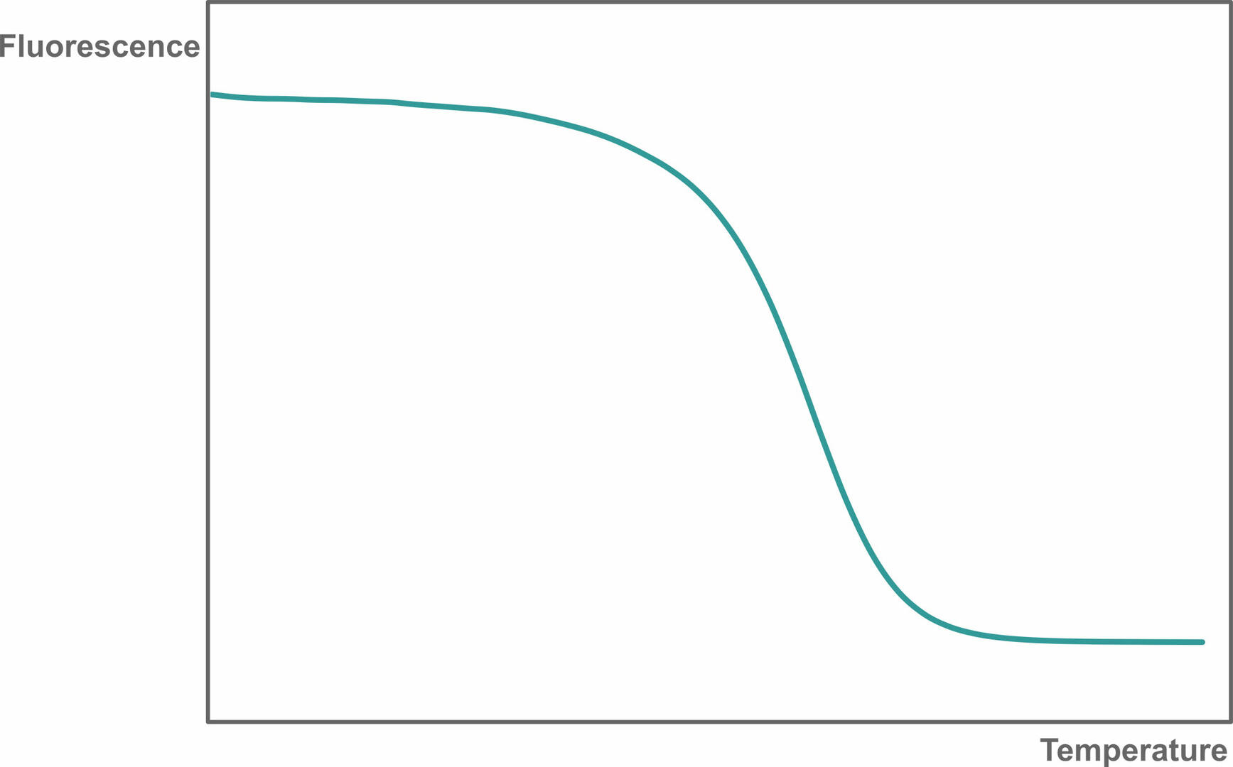
Reaction specificity can be determined using a melting curve analysis, allowing you to identify non-specific qPCR products and primer-dimers. To perform a melting curve analysis, run a qPCR assay with a fluorescent intercalating dye like SYBR Green I. After amplification, the thermal cycler increases the temperature step by step while monitoring fluorescence. As the temperature increases, the dsDNA qPCR products present will denature, resulting in a decreasing fluorescent signal:
Then, plot the change in slope of this curve as a function of temperature to obtain a melting curve:
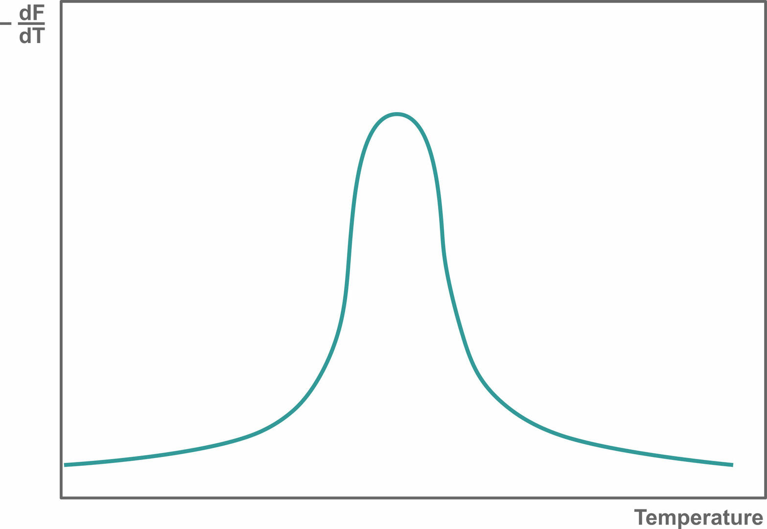
If you're observing only one melting peak like the image above, your qPCR assay is specific. If there are several melting peaks, primer-dimers and/or non-specific products were amplified during qPCR, and you should redesign your experiment to increase its specificity.
Analysis of qPCR data
qPCR data can be analyzed by absolute or relative quantification, and the method suitable for your experiment depends on your goal. Absolute quantification allows you to determine the quantity of starting material that was present in a given sample before amplification. For example, this method can be used to determine the viral load of a patient sample. Relative quantification is applied to compare levels or changes in gene expression between different samples. For example, it is helpful to investigate whether the expression of a certain gene is higher in a tumor sample than in a healthy control sample.
Absolute quantification
After qPCR amplification, you will have produced an amplification plot, and know the Ct value of each sample. To find the quantity of starting material present in your samples, you need to compare these values to a standard curve. As seen above in the section on reaction efficiency, a standard curve is obtained by amplifying a serial dilution of a sample with a known amount of template DNA, then plotting the Ct values against the log of the starting quantities.
The equation for the linear regression line of the standard curve (y = mx + b) will then allow you to calculate the quantity of starting material for each sample. As y corresponds to the Ct value, and x to the log quantity, the equation for the linear regression line is equivalent to:
Ct = m(log quantity) + b
Solving this equation for the quantity will give you the formula:
Quantity = 10((Ct-b)/m)
This will allow you to quickly determine the quantity of starting material in each sample.
Y = mx + b → Ct = m(log quantity) + b → Quantity = 10((Ct-b)/m)
Relative quantification
To compare levels or changes in target gene expression between different samples and a control sample, you first need to define a reference gene whose expression is unregulated. Then, run a qPCR to obtain the Ct values for the reference gene, target gene in your samples, and the control sample.
If the reaction or primer efficiencies for the reference and target genes are near 100 %, and within 5 % of each other, you can then use the ΔΔCt method – also called the Livak method – to determine the expression rate of the target gene in your samples. However, if the efficiencies are further apart, you should use the Pfaffl method. To learn how to calculate reaction efficiencies, please refer to the 'Reaction efficiency' section earlier in the article.
The calculations for the two methods are as follows:
ΔΔCt method
Normalize the Ct of the target gene to the Ct of the reference gene for each sample and the control sample:
ΔCt(sample) = Ct(target gene) – Ct(reference gene)
ΔCt(control) = Ct(target gene) – Ct(reference gene)
Normalize the ΔCt of each sample to the ΔCt of the control sample:
ΔΔCt(sample) = ΔCt(sample) – ΔCt(control)
Since the calculations are in logarithm base 2, you must use the following equation to get the normalized expression ratio for each sample:
Normalized expression ratio = 2-ΔΔCt(sample)
Pfaffl method
Calculate the ΔCt of the target gene for each sample:
ΔCt(target gene) = Ct(target gene in control) – Ct(target gene in sample)
Calculate the ΔCt of the reference gene for each sample:
ΔCt(reference gene) = Ct(reference gene in control) – Ct(reference gene in sample)
Calculate the normalized expression ratio for each sample:
Normalized expression ratio = ((Etarget gene)ΔCt(target gene)) / ((Ereference gene)ΔCt(reference gene))
Etarget gene: Reaction efficiency of the target gene
Ereference gene: Reaction efficiency of the reference gene
The normalized expression ratio obtained using the ΔΔCt or the Pfaffl method is the fold change of the target gene in your sample relative to the control. A normalized expression ratio of 1.2 would mean that you have a gene expression of 120 % relative to the control.
Conclusion
We hope that this blog post answered all your questions regarding qPCR methods, assay validation and data analysis. If not, please leave a comment below, and we will get back to you as soon as possible.
For questions on the ideal PCR lab set-up, primer design, or useful PCR tips and tricks, these articles could also be of interest for you: